Preparing Business Plans and Economic Feasibility Studies for Private Sector Infrastructure Provision

	Preface
	Summary
	1 Regional Infrastructure: An Overview
	2 Preparing a Business Plan
	3 Economic Evaluation
	References

Prepared by
Applied Economics Pty Ltd
Level 3, 101 Sussex Street, Sydney
Tel: (02) 9290 2498
Email: pabelson@efs.mq.edu.au

For the
Institutional Investor Information Service
Australian Council for Infrastructure Development
http://www.auscid.org.au

Preface

The preservation and development of regional infrastructure in Australia has been a particular concern in recent years. Reflecting this concern, the Commonwealth Department of Transport and Regional Services commissioned the Australian Council for Infrastructure Development (the Council) to organise a series of workshops on infrastructure development around Australia. The Council in turn commissioned Applied Economics and the Regional Institute to prepare and run the workshops.

In 2000, workshops on the development of regional infrastructure were held in the Barossa, Bendigo, Nowra, Dubbo and Townsville. These workshops discussed the nature of infrastructure, the preparation of business plans for private financial support, the preparation of cost-benefit studies to show that developments are in the public interest, the politics of gaining public support for major projects, and various local projects in each area.

Following the workshops, the Council requested Applied Economics to revise the workshop notes into a paper for general distribution via a Council website prepared by the Regional Institute. This paper is the result. As will be seen, the paper focuses on the preparation of business plans and economic evaluations rather than on political issues, important as the latter are.

It is not possible in a short paper to describe all the requirements of a business plan or an economic evaluation. Readers who require more detail may follow up the references provided or contact the writer for more information.

In preparing the paper, we acknowledge the support provided by Dennis O'Neill (Australian Council for Infrastructure Development) and Claire Braund (the Regional Institute) and the many constructive comments of participants at the workshops. However, this paper does not necessarily reflect the views of the Australian Council for Infrastructure Development or the Regional Institute. Professor Glenn Withers, a Director of Applied Economics, ACT office, also contributed to the infrastructure workshops and this paper.

Dr.Peter Abelson
Applied Economics Pty. Ltd.

Summary

This paper describes how to prepare business plans and cost-benefits studies to obtain private and public sector support for infrastructure proposals.

A business plan, including a financial feasibility study, is essential to obtaining the support of financial institutions for both debt and equity finance.

Undertaking a cost-benefit analysis is generally essential for obtaining government approval for a major infrastructure project

Section 1: Introduction

Section 1 introduces the main issues. This section outlines the nature of infrastructure, recent trends in infrastructure investment and the role of the private sector. It emphasises the dependence of infrastructure on long-term capital and the critical importance of achieving a competitive rate of return on capital employed. Unless a competitive return is expected, the private sector will not be interested in financing infrastructure. It also describes the main government policies towards infrastructure investment, especially by the private sector.

Section 2: preparing a business plan

Section 2 describes the contents required for a business plan and focuses particularly on how to make market forecasts, how to do financial analysis, organisational issues, the treatment of risk, and implementation procedures.

Market analysis includes analyses of the existing and potential feasible market size, market share, and market growth. Market size and share are often sensitive to service features and quality, household characteristics, and to price(s).

Market analysis should draw where possible on careful statistical analysis of existing data. There are often many such data for infrastructure services.

However, there are often few data on market potential or new services. Here the analysis must usually rely on household surveys generally by way of in-depth household interviews or by mass quantitative surveys, or by both methods. However, expressions of intent to purchase or use a service must be treated with caution when there is a lack of supporting behavioural evidence.

A financial feasibility analysis is based on a model of the project that simulates the revenues and costs of the business over the life of the project. The notion of discounting is fundamental to financial appraisal. This is the technique for converting streams of future net cash flows (revenues less costs) into current terms.

Discounted cash flow (DCF) analysis can be done by estimating the net present value (NPV) of a business or by estimating its internal rate of return (IRR). Both methods provide a way of assessing the total financial return on total capital employed and the return to shareholders. In both cases a critical issue is the rate of return required. The paper demonstrates how these DCF methods work.

We then describe more detailed financial issues including the profit and loss account, the balance sheet, cash flow analysis, and financial statistical analysis.

A business plan must also include an organisational structure and implementation plan. Details on the promoters' experience and expertise and financial substance and contribution to the project are especially important to financial institutions.

The implementation plan should contain specific objectives and a reasonably detailed checklist of the various steps that are going to happen in each calendar quarter.

A funding plan is required including an outline of the proposed gearing, sources of seed capital, long term equity capital, debt capital and financial assistance (if any) from the public sector.

Also a strategy for dealing with risk should be described. The business plan has to provide assurance to potential financial backers that risks have been considered and that strategies are in place to address them.

Section 3: preparing an economic evaluation (cost-benefit analysis)

Section 3 describes how to do the most common form of economic evaluation: a cost-benefit analysis (CBA). A CBA assesses the value of a business or project from the perspective of the community as a whole. It attempts to quantify all the impacts in monetary terms, although some items may be too difficult to quantify and remain 'intangibles'.

The estimated net present value of a business or project shows whether expected quantified benefits exceed expected quantified costs. Benefits represent the value of income or consumption gained; costs are the value of consumption lost. If the estimated NPV is positive, the value of aggregate income or consumption in the community is expected to increase.

The general valuation principle is willingness to pay. Services are worth the maximum that individuals are willing to pay for them. Resources used in the process are valued on the basis of what another producer is willing to pay for them.

Costs and benefits arising at different points in time are discounted to present values, generally using the social opportunity cost of capital discount rate. This is the highest rate of return that would be achieved with an alternative use of the funds.

When a project entails significant risk, the effects of these risks should be shown by sensitivity tests.

When a project has a significant impact on the distribution of welfare, especially when it has an adverse effect on low-income or other disadvantaged groups, it is important to assess the distributional impacts and consider how these can be mitigated.

In most circumstances, a cost-benefit study provides a more robust method of evaluation than the main alternatives such as cost-effectiveness analysis, GDP studies, regional economic impact studies, financial analysis, and multi-criteria analysis.

1 Regional Infrastructure: An Overview

In this first section, we discuss the nature of infrastructure, trends in infrastructure expenditure, the roles of government and the private sector, and in particular the critical role of the rate of return on capital investment.

The Nature of Infrastructure

Infrastructure typically describes a physical facility that provides basic services or inputs to a wide range of economic activities. Transport facilities, power, water and sewerage, and communications networks are classic forms of such infrastructure (sometimes called economic infrastructure). Adequate economic infrastructure is critical to the efficient functioning of most business activities.

Other forms of infrastructure include physical facilities such as schools, hospitals, prisons, community centres, libraries and recreational assets. These are sometimes described as social infrastructure. In fact, some of these facilities, notably education facilities, may also be described as economic infrastructure, as they as basic to the development and efficiency of business services.

Viewed still more generally, various other services may also be considered part of a region's economic infrastructure services. For example, law and order services, financial (banking), and legal services are all necessary requirements for sustainable economic activities.

Finally, large projects or even a cluster of projects may also be viewed as local infrastructure. For example, a large mining operation, a processing plant, or a large tourist development or marina may sustain many other local businesses.

This paper describes mainly the financial and economic requirements for developing economic infrastructure. But most of the principles and practices describes apply equally to social and other forms of infrastructure.

Economic infrastructure has several significant characteristics with implications for the method of supply.

• It often requires a large amount of capital and can take years to develop.
• It often has a long life and returns from investment can take along time.
• The physical assets may not have alternative uses or resale value.
• It often has natural monopoly characteristics (it can be supplied efficiently by only one supplier).
• It may provide significant benefits to third parties that cannot be appropriated by the owner of the physical facilities.
• It is often part of a larger network, which may complicate the analysis and necessitate negotiations between the developer of the infrastructure and the network manager.
• It often provides basic social services as well as economic services.

Because of the essential nature of the services and the monopoly nature of the production, government has traditionally been the main supplier of economic infrastructure. Because of the capital required and the length of the payback period, the private sector has been a cautious investor in infrastructure, at least without government support.

Trends in Infrastructure

In its most recent review of infrastructure capital in Austalia, the Australian Bureau of Statistics (1997) estimates that the total value of Australia's investment in economic and social infrastructure is about $400 billion-or one-third of total capital stock in Australia (Table 1.1). About two-thirds of this infrastructure is economic, the rest is social.

Table 1.1 Australia's Infrastructure (30 June 1996)

	$ bn
Private sector
Electricity, gas and water	4.9
Transport, storage and communication	30.4
Health, education, community services	18.9
Public sector
Public enterprises	171.8
General government	157.4
Total infrastructure	383.4
Total capital stock	1181.9

Source: ABS, Capital Stock, Cat.No.5521.0.

Governments own about 80% of the infrastructure. Of this, the Commonwealth owns about one-quarter and State Governments own most of the rest.

As shown in Figure 1.1, annual public investment in infrastructure fell from around 9% of gross domestic product (GDP) in the 1960s to less than 5% in the 1990s. State and local government investment fell especially, from about 7.5% of GDP to about 3.5% of GDP. Commonwealth investment was relatively steady at about 1.5% of GDP.

Figure 1.1 Public investment: Historic trends

Source: EPAC, 1995a.

As a share of GDP, economic infrastructure fell by more than half from 7.4% in 1965-66 to 3.5% in 1992-93. The decline was greatest in roads and utilities. However, some of the decline in utilities compensated for over-investment in the early 1980s. Communications and air facilities are exceptional, increasing expenditure areas. Investment in social infrastructure fell slightly from around 2.0% to about 1.5% of GDP.

This decline in infrastructure investment, which also occurred in many other developed countries, reflects several factors: economic maturity, slower population growth, and a change in the nature and composition of economic output towards more community service and knowledge-based industries that rely less on infrastructure. The decline does not necessarily indicate too little investment, though it may do.

There has moreover been an apparent decline in the proportion of infrastructure investment in regional areas, although detailed geographic data are not available. The regions have suffered from the decline in investment in roads and rail. Also, regional centres that often require upgraded infrastructure, notably for water supply, airports and telecommunications, appear to have suffered relative to metropolitan centres. Private equity investment in infrastructure has largely bypassed the regions.

Role of the Private Sector

Another trend has been the increasing role of the private sector in infrastructure, at least in the metropolitan areas. The private sector currently undertakes about a third of all investment in economic infrastructure (mainly communications, transport, electricity, gas and water industries) and a fifth of investment in social infrastructure (mainly schools and hospitals).

This trend partly reflects the sale of government infrastructure assets to the private sector. Over the last ten years, governments have sold many power generators and distributors, water utilities, rail operations, airports, gas pipelines, and nearly half of Telstra. Between 1989 and 1998, government revenue from all asset sales exceeded $61 billion.

There has also been a widespread policy shift towards increased use of private capital through a variety to mechanisms to fund new infrastructure. Build, own, operate and transfer (BOOT) schemes have been used in particular for major road, electricity and water supply infrastructure (EPAC, 1995b).

Private sector funding of new infrastructure projects has introduced economies in construction, a more innovative approach to finance and, overall, the provision of more cost-effective infrastructure. Projects are now built that otherwise, with public budget funding, would be delayed or might not occur at all.

The Australian Council for Infrastructure Development (1999) describes some of the benefits. In Victoria, Coliban Water saved an estimated 20 % of costs on both a new drinking water treatment plant and a wastewater project through its partnerships with the private sector. In NSW, private sector involvement in the Illawarra and Woronora filtration plant has provided savings of millions of dollars, brought forward the works, and delivered the projects with minimal impact on Sydney Water's cash flow.

More extensive examples of the benefits of private sector involvement in the provision of infrastructure can be found internationally. Details of the benefits in the UK, for example, can be found under the UK Treasury website, http://www.treasury-projects-taskforce.gov.uk

Table 1.2 shows a variety of private funding arrangements for infrastructure. In addition, service contracts, such as water filtration and maintenance, are often out-sourced.

Table 1.2 Guide to Private Involvement in Economic Infrastructure

Areas of involvement	Full private ownership	BOOT-type arrangements			Public ownership with contracting out	Traditional public ownership
		BOO	BOOT	BTO
Plan	P	G	G	G	G	G
Design	P	P	P	P	P/G	G
Construct	P	P	P	P	P/G	G
Operate/maintain	P	P	P	P	P/G	G
Ownership	P	P	P_G	G	G	G
Payment for services	C/G	C/G	C/G	C/G	C/G	C/G
Regulate	G	G	G	G	G	G

Key: P = private; G = Government; C = Consumers.

Source: EPAC, 1995b.

Rates of Return on Capital

The private sector will fund an infrastructure project only if the expected return on capital employed is as high as in other economic businesses after due allowance for risk.

In order to estimate the rate of return it is necessary to forecast all revenues and cash costs (including capital expenditure) over the lifetime of the infrastructure and to discount the net operating cash flow back to the present. This form of analysis is known as discounted cash flow analysis (see Section 2).

Target rates of return are a matter of considerable controversy especially in the utility (power and water sector) that is subject to government regulation. Table 1.3 shows typical nominal rate of return targets suggested by the Commonwealth Competitive Neutrality Complaints Office in 1998. Of course, two years on, the bond rate is 6.25%.

Table 1.3 Typical nominal pre-tax rate of return targets

Level of risk	With bond rate of 5%	As premium over bond rate
Low	8	Bond rate + 3%
Medium	10	Bond rate + 5%
High	12	Bond rate + 7%

Source: Commonwealth Competitive Neutrality Complaints Office (1998)

Some infrastructure projects have little market risk because they supply essential services and face limited competition. Once established, such businesses can attract capital at quite low risk rates. The Office of the Regulator General in Victoria (1998) and the Independent Pricing and Regulatory Tribunal in New South Wales (1998) argued that a rate of return of only 120 basis points (1.2 %) above the bond rate should be adequate to compensate (and to attract) private capital in such cases. However, it is questionable whether the markets consider that this is an adequate premium even for low risk businesses.

Other infrastructure projects have large capital requirements and a long gestation period before they produce profits. They also face potential regulatory problems. Therefore they are not usually regarded as low risk ventures, at least until they are well established.

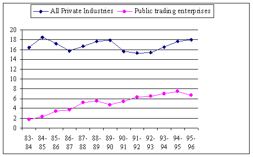
Figure 1.2 shows the financial net rates of return that have been achieved by private corporations compared with public trading enterprises. The net return is the ratio of net operating surplus to net capital stock. As discussed in Section 2, this ratio must be treated cautiously as it represents short-term results and is based on accounting conventions that do not necessarily provide an accurate measure of full economic return.

Nevertheless the results are revealing. The average rate of return has generally been much higher in conventional private markets than in public infrastructure, although the gap is narrowing. This poses a difficulty for private finance unless the lower return is offset by greater security and reduced risk.

Of course, in so far as returns to infrastructure spending flow to the community and are not captured in the rate of return to the investor, there may be a case for a public financial input. However, in developing a case for public support for a mainly private investment, the community benefit needs to be documented convincingly.

Figure 1.2 Financial net rates of return to private and public investment

Source: ABS, Capital Stock, Cat. No. 5221.0.

Sources of Private Finance for Long-Term Capital

Businesses have short, medium and long-term capital needs. A key to financial planning is to match the terms of finance to the needs: short-term finance for short-term trading needs and long-term finance for long-lived assets. The focus here is on major long-term capital needs for investment in new assets.

Long-term private sector funding generally consists of debt and equity. Projects promising robust net cash flows with relatively small risk can achieve gearing levels of up 70% debt and 30% equity in their capital structure. As a project's firm net cash flows fall, especially in the short term, and as risk rises, the level of debt falls and the more equity is required.

The main sources of debt for private infrastructure projects in Australia are the major Australian commercial banks. These banks have responded to changes in the market by, for example, increasing their lending terms to 15 to 18 years. They are also developing their capacity to underwrite inflation-indexed bonds and other long-term investments. An involvement by Australian banks is generally necessary to give comfort to overseas providers. Overseas banks, particularly UK, Swiss, German and French banks, also provide debt for major projects.

Non-bank financial institutions, such as superannuation funds, life offices and funds managers in the infrastructure area, are becoming increasingly involved in funding infrastructure. This is natural as many such funds have long-term liabilities. However, there are sometimes concerns about the illiquid nature of the financial investment.

Equity for infrastructure projects usually combines 'active' and 'passive' equity sources. 'Active or smart' equity money typically comes from an experienced operator in the industry, for example for a water project it could be CGE (France) or Thames Water (UK). The active source might supply seed equity for the initial development phase of the project, may supply wrap-around completion and performance guarantees, and could manage both the project's development and operating phases. The presence of such an experienced investor providing risk capital engenders confidence in other equity and debt providers.

'Passive or dumb' equity providers are so called because they are not experts in the industry. They draw confidence and follow on from the provision of 'smart hurt' money from substantial and expert project sponsors. Typical 'passive' equity providers for infrastructure projects in Australia include:

• Major Life Offices e.g. AMP.
• Major Superannuation Funds Managers e.g. BT Funds Managers.
• Dedicated infrastructure funds e.g. Macquarie Infrastructure Trust, Lend Lease, Hastings.

Some special funds targeting infrastructure have emerged. These funds identify and analyse infrastructure investment opportunities and raise capital for them. Examples are the Hastings Fund Management (a Utilities Trust), GELLCO Infrastructure Services (a joint venture of Lend Lease and General Electric), and the Develop Australia Fund (managed by AMP).

The first public listing of an infrastructure project was the M2 Motorway project in Sydney. This form of investment is more liquid than unlisted projects. However, direct access to the capital markets has not developed significantly for smaller infrastructure projects.

Inflation indexed bonds were used to finance the Sydney Harbour Tunnel. Using these bonds, interest payments are indexed to protect investors against inflation., However, sale of project bonds has not been used much to-date.

Government Policies for Private Involvement in Infrastructure

Although Commonwealth and State Government policies for private sector involvement in public infrastructure vary in details, there is substantial agreement on the main procedures and principles.

Implementation procedures generally include the following steps:

• Project definition generally starts with government strategic planning and initial project development.
• However, unsolicited proposals may be accepted if they fall within government planning guidelines;
• Calls for competitive proposals are followed by evaluation and short-listing of proponents;
• Proponents prepare detailed proposals. These must demonstrate that the project is in the community interest, and assessment;
• The government negotiates with the preferred proponent and a contractual agreement is prepared; and
• Ideally there would be public disclosure and implementation: public issue of a contract summary, project implementation and post-implementation review.

General principles

Common general principles are probity, transparency, accountability, and protection of the interest of the community. Private infrastructure projects can generate considerable political interest and the need for a clear and accountable process is paramount.

The chief means for achieving these processes is competition. All states have signed the Competition Principles Agreement with the Commonwealth. This agreement requires:

• Independent prices oversight of public monopolies;
• Competitive neutrality between public and private businesses;
• Structural reform of public monopolies to facilitate competition;
• Review and reform of anti-competitive legislation;
• Third party access to significant infrastructure facilities; and
• Application of these principles to local council's business activities.

These principles apply regardless of whether the public or private sector develops infrastructure. Proponents must show that the project is in the public interest, usually by supplying both an economic (cost-benefit) evaluation and an environmental impact assessment.

Three common specific principles should also be highlighted.

Commercial viability

The project must function either as a stand-alone commercial undertaking or through fee for service income from the Government. Most governments require that investment in infrastructure is justified by economic evaluation of the merits of the case (EPAC, 1995b). In the words of the National Commission of Audit (1996), economic rates of return on infrastructure `provide the best guide to the merits of any particular infrastructure project'.

Of course, this rate of the return should include any benefits to third parties (see Section 3 below). For example, privately financed roads may reduce congestion on the public road system.

Moreover, social considerations may justify additional investment in infrastructure. For example, all Australian citizens may be regarded as entitled to certain service levels for education, health, communications, water supply and so on. It is the job of government to decide what these service levels should be and to determine the subsidies (community service obligations), if any, that are required. Once this subsidy is identified, it can be included in business plans and economic feasibility studies.

However, infrastructure cannot be justified by vague or general arguments that infrastructure is necessary for development or that it creates multiplier benefits in the form of additional local income and employment. Useless activities, like digging holes in the ground and then filling up the holes, create multiplier benefits. (For further discussion of multiplier effects, see Section 3). The argument that infrastructure creates more flow-on benefits than other investment has little support among academic economists, national Treasuries (BTCE, 1996), or international financial institutions (World Bank, 1994).

Cost-effectiveness

Even if a private proponent develops a new concept, the proponent must show that their group is the best-equipped and most efficient agency to carry out the project. Involvement of the private sector must achieve net efficiencies in financing or construction or operational aspects of a project relative to public sector provision. Most governments favour private sector involvement. However, this must be demonstrated to be in the public interest.

Most governments favour competitive tendering. Occasionally, government awards an exclusive mandate for an unsolicited proposal, often for political reasons. However, this raises issues of transparency, equity and probity.

Most governments are cautious about allowing private firms to run public monopolies. Swapping state-owned monopolies for private ones has been avoided through creation of markets where previously none existed, such as for electricity; by licensing new entrants, as in telecommunications; and by curbing monopolistic opportunity through regulation, as for high voltage transmission systems. This is achieved by retaining control of pricing through the national regulatory agency, the Australian Competition and Consumer Commission. Competition promotes efficiency, choice and innovation. This is evident in both the telecommunication and power markets following the privatisations in the mid-1990s.

Risk-sharing.

Most state governments are keen to ensure that projects are structured to limit their exposure to risk. Where the private sector seeks to retain the returns accruing from infrastructure provision, it is generally required to take the associated risks of such projects.

Other government policies

Other government policies that have a substantial impact on infrastructure provision are public finance and tax initiatives.

At the Commonwealth level, the Department of Industry, Science and Resources has established initiatives to improve the availability of equity based finance to business. Invest Australia is a national investment agency designed to attract foreign investment to Australia. Finance initiatives managed by Invest Australia include Pooled Development Funds that aim to develop patient equity capital for small and medium sized enterprises and the Innovation Investment Fund that encourages early-stage development companies.

Some States have established infrastructure funds. For example the Victorian government set up a regional infrastructure development fund with $170 million funding in November 1999. The Queensland Investment Incentive Scheme allows for targeted government financial support, for example with favourable tax treatments, to influence the location of important projects. Interested parties should investigate the availability of state funds from relevant state agencies.

Tax issues are complex. There has been concern for some time that private investment in infrastructure is discouraged because depreciation allowances are inadequate and because of restrictions on deductions of losses from other taxable income. There are related concerns about the operation of the anti-tax avoidance provisions in Section 51 AD and Division 16D of the Income Tax Assessment Act. On the other hand, the Infrastructure Borrowings Tax Offset Scheme is limited in both scale (to $75 million a year for five years) and scope (to land transport infrastructure).

More details of the debate on financing and tax issues can be found in Australian Council for Infrastructure Development (1999) and in the report of the Standing Committee on Primary Industries and Regional Services (2000, Chapter 4).

Final Comment

The key economic issues for infrastructure investment are the financial return to private investors and the social rate of return to the community from investment in infrastructure. In the long run, these must be competitive to attract private or public capital respectively.

2 Preparing a Business Plan

This section outlines the main components of a business plan, some key elements of market analysis, how to do financial analysis, and the important issues of organisation and risk management.

Introduction

A formal business plan is essential to a successful project. As venture capitalist Chris Golis (1998) observes, just as it would be folly to renovate a house without architectural drawings, so an investor would be foolish to invest in a business without a formal business plan.

A business plan must be a written document. It is easier to talk about a concept than to write about it. The written business plan is the finished product. When the concept is down on paper it is easier to analyse, change and improve.

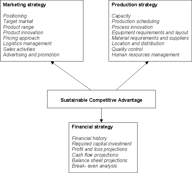
As shown in Figure 2.1, a business plan has three major functional elements: a marketing strategy, a production strategy and a financial strategy. In more detail, most plans should address the areas shown in Box 2.1.

Box 2.1 Main components of a Business Plan

I	Executive summary
II	Business description
		Business definition
		Product / service definition
		Industry relationships
III	Market analysis
		Market definition
		Market positioning
		Pricing strategies
		Distribution strategies
		Sales strategies
		Competitive analysis
IV	Design and development
		Development plan
		Timetable, priorities and key milestones
		Costs of development
V	Operations and management plans
		Management structure
		Operational methods and input requirements
		Human resources management
VI	Financial analysis
		Overall financial analysis
		Funding proposals
		Profit and loss and balance sheets
		Financial analysis tools
VII	Summary
		Key indicators
		Risk analysis
		Action plan

Figure 2.1 Major elements of a business plan

Source: Ausinfo, 1998.

Of course, the structure and detail in business plans may vary not only between businesses but also as a plan is developed for a business.

In the first instance, it is common to undertake a SWOT analysis-an analysis of business's strengths, weaknesses, opportunities and threats. This analysis is generally qualitative rather than quantitative. It helps to identify the core basis, rationale and sustainable competitive advantage of a proposed business.

After the initial examination of prospects, the business plan should progressively detail and quantify the proposal. Quantitative performance measures must be established to support the set objectives.

In this discussion, we focus on three main issues: market analysis, financial analysis, and project organisation, operation and risk.

In order to illustrate some of these issues, we refer in this and the next section to a hypothetical high-speed rail project from Sydney to Canberra. There have been several studies of this project. However, the example given here is hypothetical. It does not purport to describe any existing proposal and the figures should not be used to infer likely costs, benefits or outcomes of any actual proposal.

Market Analysis

Market analysis is the basis of all business plans. The market analysis must clearly show the market opportunities, key features of the market, market dynamics, the competition, and the key success factors in the industry.

Market analysis typically consists of three estimates: (i) market size, (ii) market share, and (iii) growth prospects. If one business may capture most of the market, as it may for some infrastructure services, it may be appropriate simply to estimate (i) the expected market for the business and (ii) the growth of this market. However, we follow below the usual threefold structure of market analysis.

Estimating market size

Market size includes existing and potential users of a service. Because of the basic nature of infrastructure, there is often an existing service, for example for water or electricity, where sales or consumption are well known. Likewise, existing services for health or education are usually well known.

However, current sales or services used depend on the quality of the service and on prices. The potential market may be much larger than existing sales. In the transport sector, for example, some people may be deterred from travelling by the poor quality of the road infrastructure or by the high prices of airline services. Estimates of market size should show how services demanded would respond to changes in service quality and prices. This usually requires either statistical analysis of consumer behaviour in different circumstances or household surveys.

On the other hand, there is a danger that estimates of potential market size may overestimate the feasible market. The feasible market is a function of market segmentation. It is important to know who is using, or likely to use, the service. Thus the feasible market could be a certain percentage of households who live in particular areas, who have a certain income, who have cars, or who have children and so on. The market analysis should show therefore how consumption varies with household size, age composition, income and other household attributes. Estimates of the potential market should take into account these constraints on market size.

Box 2.2 Total Market for High Speed Rail from Sydney-Canberra Train

The market for high-speed rail travel from Sydney to Canberra consists of existing and potential trips for passengers and freight between (i) the two cities and (ii) intervening towns. Existing trips include rail, air and road (car and coach) journeys. Data on air and rail trips between Sydney and Canberra are readily available. However, to estimate the road trips between Sydney and Canberra that might divert to rail, data on trip lengths, origins and destinations are needed. This requires a special survey of road users. To estimate the total potential passenger market for the high-speed rail, we need to know how many extra trips will be made as a result of the new travel mode. This depends on consumer responses to savings in travel times and attitudes towards different modes of travel. A high-speed train could reduce rail line haul times between Sydney and Canberra from eight to two hours. However trip decisions depend on door-to-door travel time, which varies greatly with origin and destination. Therefore, data are needed on origins and destinations and on the sensitivity of trip decisions to journey time. The potential market will also depend on the rail fares of the proposed new service. There may be some generated freight market due to the faster train. However, not many freights are highly time sensitive - and there is an air alternative.

Establishing market share

The key factor in determining market share is competitiveness. Few services are immune from competitive threat. For example, only one airport may directly serve a town, but another one may provide indirect (road plus air services) and competitive frequencies. Gas competes with electricity, and so on.

Although many infrastructure services, such as water and power, provide a more or less standard product, the products often have different features that households value. For example, some people prefer to cook with gas rather than electricity. Some consumers value the flexibility of the private motor vehicle compared with use of public transport. It is important to identify as precisely as possible the features of a product that firms or consumers value.

Pricing is often critical to market share. The more similar are the products to those of competitors, the more sensitive is market share to price. The sensitivity of demand to price is measured by the price elasticity of demand. Demand is said to be sensitive to price (price elastic) if consumption changes (inversely) more than proportionally with price changes. Demand is insensitive (price inelastic) if consumption changes (inversely) less than proportionally with price changes.

Of course, market share depends on relative prices. It is dangerous to assume other prices will stay constant or that, if your business cuts prices, competitors will not react with their own price cuts. In the long run, prices are likely to reflect (i) relative product quality and (ii) production costs. The safest long-term assumption to make is that competitors will price their services to cover their long-run costs.

However, it is important not to place too much emphasis on market share. What matters (financially) is net revenue. When demand is not responsive to price cuts, increasing market share by reducing prices reduces gross revenue, and increases operating costs.

Also converting potential purchasers into actual ones takes time. It often takes a few years to reach the full competitive market share for a product.

On the other hand, few competitive advantages last for a long time. Estimates of market share should recognise that competitors may develop new or more competitive services over time.

As part of the analysis of market share, a business plan should describe the marketing strategy that will be required to obtain and sustain the market share.

Box 2.3 Market Share for High Speed Rail from Sydney-Canberra Train

To estimate market share, it is necessary to estimate the diversions from rail, air and road, as well as the potential expansion of the market due to the new service. Over 80% of trips from Sydney to Canberra trips are by road, so diversions of road trips are a major issue. Diversions from rail depend on service availability and fares. If the public rail service continues to operate with a large subsidy, existing passengers (mainly pensioners and children) are unlikely to be willing to pay a fivefold increase in fares, from say $10 to $50 per trip, for the savings in travel time. However, government may prefer to pay the new rail operator a community service payment to provide the rail services rather than provide its own subsidised service. Diversions from air depend principally on savings in travel time and fares. These savings depend on the door-to-door trip logistics and costs and on how airlines respond with lower airfares or other services to the increase in competition. Diversions from motor vehicles depend on numerous factors. The number of passengers per road vehicle is particularly important because this affects average trip cost. Also, trip purpose matter, because some trips have multiple purposes or stops. Diversion rates will also be sensitive to origins and destinations, rail price, service frequency and quality. Detailed survey work is required to estimate these diversions from road trips.

Market growth rate

Many forecasts of market growth draw on past growth rates. The simpler forms of forecast simply project the past growth for the service. However, even these forecast methods can use quite complex statistical methods (including non-linear formulations) to interpret the past trend and to project it.

Alternatively, market growth may be related to causal factors. Here it is convenient to distinguish between services provided to households (final demand) and to businesses (intermediate demand). Taking household services first, three factors are often important: demographics, household income, and future prices.

Population growth (natural or via migration) is a key driver of household demand. But most services depend on the demands of particular sections of the community, such as students or the aged. It is important to forecast the appropriate household categories.

Second, demand depends on household income. The demand for some products, such as travel, grows faster than income. The demand for others, such as water, generally increases more slowly than income. The responsiveness (or sensitivity) of demand to income growth is known as the income elasticity of demand.

Demand is said to be sensitive to income (income elastic) if consumption changes more than proportionally with income changes. It is insensitive to income (income inelastic) if consumption changes less than proportionally with price changes.

The third main factor is prices. Consumption will grow faster if industry prices are expected to fall relative to other sectors, as has happened with telecommunications.

When a service is provided to industry, industry demand for the service will depend on (i) the growth of the industry sectors that use the service and (ii) whether the service provided will become more or less important to the industry, depending especially on technical change and relative prices.

Finally there is the product cycle. Typically, industries go through various stages: establishment, growth, maturity and decline. These stages reflect the technology and competitiveness of the industry. If the quality of the infrastructure is maintained, the product cycle is usually less important for essential infrastructure services than for other industries. But even infrastructure services may not be immune from the product cycle.

Box 2.4 Market Growth for High Speed Rail from Sydney-Canberra Train

For a new product like a high-speed rail, it is not possible to extrapolate growth trends from past growth rates. In this case, the market growth for high-speed rail can be estimated as a function of the growth rates of the rival modes from which rail passengers are expected to divert. Thus numbers diverting from existing rail, air and road modes would be expected to increase with the forecast growth in rail, air and road trips. Because the growth in air and road trips is greater than income (ie. the demand is income elastic), growth rates for these diverters would be high. Because rail trips usually do not rise very fast, the growth rate for diverters from existing rail service would be low. This assumes that the relative attractiveness of travel by high-speed rail and competitive modes stays constant. Changes in relative attractiveness, for example improvements in motor vehicles, could affect the assumption that the market for high-speed rail will grow at the same rate as the markets of its competitors.

Concluding Comments

Market analysis includes analyses of the existing and potential feasible market size, market share, and market growth. Market size and share are often sensitive to service features and quality, household characteristics, and to price(s).

Market analysis should draw where possible on careful statistical analysis of existing data. There are often many such data for infrastructure services.

However, there are often few data on market potential or new services. Here the analysis must usually rely on household surveys generally by way of in-depth household interviews or by mass quantitative surveys, or by both methods. However, expressions of intent to purchase or use a service must be treated with caution when there is a lack of supporting behavioural evidence.

Financial Analysis

The financial analysis is the engine of the business plan. It is the means by which the marketing and production strategies are implemented.

Infrastructure businesses are characterised by high capital expenditures. There are therefore two key financial issues: one for equity investors and one for lenders of debt.

1. Can the business generate sufficient net cash flows to achieve a satisfactory rate of return on total capital employed, including interest capitalised during development, thus satisfying equity investors?
2. Are project cash flows sufficiently robust under adverse circumstances to provide healthy debt service cover ratios to lenders?

As we saw in Section 1, the return on capital employed is often calculated simply by dividing the most recent annual profit earned by a business by the capital employed in that business. However, this ratio is an accounting measure usually based on historic prices rather than the current value of capital employed. Moreover, it measures only the short-term return on capital. It does not guarantee that the long-term return is satisfactory, which is particularly important for infrastructure.

A financial feasibility analysis is based on a model of the project that simulates the revenues and costs over the life of the project. The notion of discounting is fundamental to financial appraisal. This is the technique for converting streams of future net cash flows (revenues less costs) into current terms.

We start therefore by describing discounted cash flow (DCF) analysis. We then describe more detailed financial issues including the profit and loss account, balance sheet, cash flow analysis, and statistical financial analysis.

Long-term discounted cash flow analysis

DCF analysis can be done in one of two ways: by estimating the net present value (NPV) of a business or by estimating its internal rate of return (IRR). We look at these in turn.

Both forms of DCF analysis require an estimate of the cost of capital to the business. This typically depends on the amount of debt and equity and the costs of debt and equity to the business. Ignoring complications of tax and dividend franking, the weighted average cost of capital (WACC) can be expressed as:

WACC = rd . wd + re . we

(2.1)

where r_d and r_e are the rates of return required for debt and equity respectively and w_d and w_e are the proportions of debt and equity used in the business (which add up to 1.0). For example, if a business is financed half by debt and half by equity, and the cost of debt and equity is 8% and 14% respectively, then:

WACC = (8.0 × 0.5) + (14.0 × 0.5) = 11%

(2.2)

Note that these rates of interest would typically be market rates that include an allowance for inflation.

If net cash flows are assumed to arise at the end of each year, the net present value (NPV) of the business is given by:

NPV = NCF/(1+WACC) + NCF2/(1+WACC)2 ...+ NCFn/(1+WACC)n (2.3)

where NCF is net cash flow and the business has a life of n years. Equation (2.3) can be adjusted if revenues or costs arise earlier in the year.

The net present value of a business is the present value of all future net cash flows. It is the value of the business. If the estimated NPV is greater than zero, the business is expected to generate sufficient revenue to provide a rate of return on capital in excess of the cost of capital over the life of the project. A simple example of a financial evaluation is shown in Box 2.5.

Equation (2.3) can be estimated allowing for expected inflation in costs and revenues and using market rates of interest that allow for inflation. Alternatively, Equation (2.3) can be estimated using constant year 2000 dollars (with no inflation) and with an inflation-free discount rate. The latter discount rate is approximately equal to the weighted average cost of capital less the expected rate of inflation. For example, if the nominal borrowing rate is 11% and inflation is 3%, the inflation free rate is approximately 8%.

It is not necessary to include inflation. It may be more practical to estimate all revenues and costs using constant dollar values and an inflation-free discount rate. The two approaches (working with and without inflation) give similar results if taxation is ignored (see Box 2.5).

Box 2.5 Example of a simple financial evaluation

Scenario A: a proposed investment has (a) a capital cost of $50 million, (b) net revenues of $7.0 million per annum for 10 years, (c) a residual asset value of $10 million. All monies are in constant year 2000 dollars, all monies are spent and received at the end of each year, and the average real rate of return required is 7 per cent. The total net return is $3.7 million and the investment is financially viable. Scenario B: the same basic values are assumed, but there is an inflation rate of 3% per annum. The rate of return now required is 10.21% (1.07 × 1.03 = 1.1021). The total net return is again $3.7 million.
Year	Scenario A	Scenario B
	($m)	($m)
1	-50.0 / 1.070	-51.3 / 1.102
2	7.0 / 1.145	7.4 / 1.215
3	7.0 / 1.225	7.6 / 1.339
4	7.0 / 1.310	7.9 / 1.475
5	7.0 / 1.403	8.1 / 1.626
6	7.0 / 1.501	8.4 / 1.792
7	7.0 / 1.606	8.6 / 1.974
8	7.0 / 1.718	8.9 / 2.176
9	7.0 / 1.839	9.1 / 2.398
10	7.0 / 1.967	9.4 / 2.448
11	7.0 / 2.105	9.7 / 2.699
12	10.0 / 2.252	14.3 / 2.974
Total net revenue	3.7	3.7

An alternative form of discounted cash flow analysis is internal rate of return (IRR) analysis of the free cash flow. The IRR is the discount rate that will produce an NPV of zero. In this case, we can write

0 = NCF/(1+i) + NCF2/(1+i)2 ... NCFn/(1+i)n

(2.4)

where i is the internal rate of return. The value of i has to be calculated; it is not known in advance. If the estimated IRR exceeds the average cost of capital for the business, the business is expected to be viable.

Of course, this also means that the net present value of the business will be positive. In Section 3, we discuss some special cases when the NPV and IRR estimates give conflicting answers.

The discounted cash flow analysis for a hypothetical Sydney-Canberra high-speed train illustrates the approach. The analysis allows for a 3% rate of inflation and assumes an average cost of capital of 11% in nominal terms. The inputs to this simplified financial analysis are shown in Box 2.6.

Box 2.6 Hypothetical Sydney-Canberra high-speed train: inputs to financial analysis

Expenditures (in year 2000 dollars)
Capital track/station costs	$3000m over five years
Rolling stock	$ 200m in year 5, $100m in year 20
Track and plant maintenance	$ 10m p.a.
Fixed annual costsa	$ 20m p.a
Variable costsb	$ 12 per passenger trip (average)
Revenues (in year 2000 dollars)
Passenger trips (Sydney - Canberra)	2.0m in opening year
Passenger trips (intermediate trips)	0.5m in opening year
Annual growth in passengers	3% p.a.
Passenger fares	$55 per single full trip
	$15 per intermediate trip
CSO paymentsc	$25m p.a.
Other revenuesd	$5m p.a.
Residual sale valuee	66% of capital costs
Assumptions
Inflation 3% p.a. Weighted average cost of capital 11% p.a.

(a) Include overheads, administration, marketing, payments to NSW rail agencies etc

(b) Include train operating costs, labour, materials, energy etc

(c) Community service payments by government as subsidies for pensioners and students.
(d) Revenues from stations, advertising etc.
(e) At end of 30 years of operation.

The details and results of the financial analysis are shown in Table 2.1. On the basis of the assumed figures, the estimated net present value of the hypothetical high-speed train (the capitalised value of the losses) would be -$1.5 billion. The estimated rate of return on capital employed is 5.3% compared with an assumed weighted average cost of capital of 11%. On these assumptions, the hypothetical high-speed rail would not be financially viable. It would have to be justified on broader cost-benefit grounds (see Section 3).

The financial analysis could be remodelled to include all financial flows to the proponent. For example, it could include loan receipts and repayments of debt principal and interest. However, if this were done, it would essentially be a model of the project from the perspective of the equity investors. As we saw above, equity investors are likely to require a higher return on capital than debt providers.

More detailed financial issues

Turning to more detailed financial issues, a business plan should contain forecasts of the:

• profit and loss account (income statements),
• balance sheet (showing assets and liabilities), and
• cash-flows.

Examples of each of these (sourced from Ausinfo, 1998) are shown at the end of this section. Typically a business plan would contain forecasts of profit and loss, net assets and cash flows for at least the first 3-5 years of operation.

The profit and loss account shows gross and net profits, or losses, on an annual basis. The following are some of the key indicators contained in the account.

• Gross profit (GP) = sales - variable cost of goods sold.
• Operating profit = GP - fixed costs = earnings before interest and taxation (EBIT).
• Net profit before tax = EBIT - interest payments.
• Post-tax profit = net profit before tax - tax payments.

The balance sheet of a company describes how much capital is employed in a business and how it is distributed among the various assets. Some key figures and relationships are:

• Capital employed = shareholders equity + net loans
• Total assets = current + non-current assets
• Net assets = total assets - current liabilities = capital employed
• Shareholders equity = capital employed - net loans

Note that a balance sheet prepared for a business plan may be different from one prepared for statutory purposes. A business plan will show total capital employed and shareholders equity and the estimated return to all funds to be employed by a business as well as the return to equity holders. The balance sheet, together with the profit and loss statement, should show how this occurs. A statutory balance sheet is more limited: it reports to shareholders about the past.

Thirdly, a business plan must show how cash flows will be managed. This means allowing realistic timing for all expenditures and receipts, estimating the working capital required, and showing how cash deficits are to be financed. The cash flow, or flow of funds, analysis will therefore show:

• capital expenditure,
• capital financing cash flows (debt, equity), and
• operating cash in (sales, royalties, etc.),
• operating cash out (material, labour, rents, tax, etc.),
• interest and dividend payments,
• changes in net loans.

Statistical financial analysis

The business plan should also report on key financial ratios that financial institutions expect to see. Of course, insofar as the ratios are derived from the profit and loss account or balance sheet, the institutions could make the calculations themselves. However, it is good practice to make these ratios explicit.

For investors in infrastructure projects, the major concern is the long-term return on capital employed. However, the following ratios are also likely to be of interest:

Break-even point: The point at which sales recover all operating costs and costs of goods and start to make a contribution to debt repayment.

Gearing ratios: The debt-equity ratio is expressed as the percentage that total debt represents of shareholders' funds. The larger the ratio, the smaller the protection given to lenders by the availability of shareholders funds (net business assets).

Return on equity: the return on equity equals post-tax profits divided by shareholders funds expressed as a percentage. As a rule of thumb, to attract private investors, the nominal return on equity should be at least 15% unless expected inflation is very low.

Debt service cover ratio (DSCR): this is of fundamental concern to financiers. A commonly accepted definition is:

Lenders will set minimum cover ratios to reflect the perceived riskiness of the project. Indicative range for minimum required DSCRs on a base case (most likely case) scenario would be 1.5 to 2.5. Financiers will seek DSCRs in excess of 1.0 across a range of possible adverse scenarios to ensure the project cash flows are sufficiently robust to service debt obligations and that the probability of loan default is low (indicatively less than 1 per cent).

Organisation, Risks and Actions

The operational and organisational issues of importance to investors comprise another significant part of a business plan. Among these issues are the organisational structure, quality of management, environmental threats, and implementation plan.

Financiers need details of the company, organisation or people promoting the project. In particular, they will seek information about:

• The promoters' experience and expertise in successful developments of this nature;
• The financial substance of the promoters; and
• Assets and resources being supplied by the promoters to the project.

The business plan should describe the corporate structure. These structures for infrastructure projects are often complex because of the need to address such issues as tolling arrangements to capture revenue, risk apportionment, guarantees and financiers' security concerns.

Another key task is organisation of the management team. This team should include people with skills in product development and operations, administration, finance and marketing.

Risk assessment and policies

A risk assessment analysis should identify the key risks facing the business in both the development and operating phases. The assessment should also show how risk is allocated to participants and how the business's strategic plan will neutralise the various possible risks.

The following are some risks that should be considered (Treasury, Victoria, 1998).

• Completion risk covers all potential for cost and time overruns incurred in tendering, planning approvals, design, engineering and construction.
• Operating risk covers potential risks in technical and operating performance, efficiency, management capability, contract management, technology and obsolesence.
• Market and demand risk arises when there are significant uncertainties in markets.
• Sponsor risk relates to areas relevant to the project sponsor's experience and expertise, such as credit strength and commitment to the project.
• External risks are risks outside the control of the parties involved in the project, including changes in financial markets and cost of capital, general taxation risks, environmental threats, and acts of God (floods, earthquakes and so on).
• Sovereign risk covers those risks affecting the delivery of a project resulting from changes in government policy or regulations.
• Contract termination risk covers the possibility that the value of an asset may not reach its expected value at the end of the contracted term.

A traditional obstacle to private infrastructure funding in Australia has been concern on the security of the Government concession or licence in the event of a service failure. Banks in particular need the comfort that, in the event of project difficulties, the Government concession or licence will survive so that they may work though the difficulty to get their money back.

Formally, risks may be assessed quantitatively (usually by sensitivity analysis) or qualitatively (by expert judgement). Using sensitivity analysis, the analyst considers the range of possible values for the important assumptions and estimates the effects of changes in these values on the financial outcome. Financial institutions can then judge whether the expected rate of return is higher enough to justify the risks involved.

Alternatively, the proposal may have to be modified to reduce the risks. In any event, the business plan should describe the proposed actions to avoid or mitigate risks.

Implementation plan

Finally, a business plan must include an implementation plan. This should start with a statement of the two or three key objectives the business will accomplish in each of the next two to three years. The plan should then contain a reasonably detailed checklist of the various steps that are going to happen in each calendar quarter.

Critical inputs to implementation are plans for funding and for handling risk. A funding plan is required including an outline of the proposed gearing, sources of seed capital, long term equity capital, debt capital and financial assistance from the public sector.

A strategy for dealing with risk should be described. The business plan has to provide assurance to potential financial backers that risks have been considered and that strategies are in place to address them.

Source: Ausinfo, 1998.

Source: Ausinfo, 1998.

Source: Ausinfo, 1998.

3 Economic Evaluation

An economic evaluation generally assesses the value of a business or project from the perspective of the community as a whole. It is thus differs from a financial evaluation that assesses the value of a business or project from the perspective of the providers of finance.

For most purposes, economic evaluation is synonymous with cost-benefit analysis (CBA). CBA attempts to quantify all the costs and benefits of a project to whomsoever they accrue. The economic evaluation method most commonly required by governments in Australia and elsewhere is cost-benefit analysis (Department of Finance, 1991).

This section of the paper describes the main steps in a cost-benefit analysis, the decision framework, how to value costs and benefits, and the treatment of distributional issues. The last substantive section compares CBA with some alternative methods of evaluation.

Steps in Cost-Benefit Analysis

Box 3.1 outlines the main steps in a cost-benefit analysis. These steps follow the normal processes in policy determination. The main difference in CBA is the formal and rigorous approach to assessing the consequences of the options.

Box 3.1 Key Steps in Cost-Benefit Process

Identifying issues and objectives

The starting point for any project should be a clear statement of the problem to be addressed and the objectives to be achieved.

It is important to focus on the problem to be solved. For example, the capacity problem at Sydney's Kingsford Smith airport is essentially one of excess demand for runway capacity at peak hours caused mainly by small aircraft on domestic flights. The issue is therefore how to provide more runway capacity in the Sydney basin for these aircraft. The answer is not necessarily a new international airport with two long, wide-spaced, parallel runways.

Objectives should be defined in terms of specific and measurable outcomes, such as improvements in travel times, water quality objectives, or health status achievements. There should be a clear statement of the numbers of people who may benefit. Projects must be justified ultimately by the delivery of specific services to individuals.

Developing options

A range of possible options for solving the problem(s) and meeting objectives should be considered at an early stage in the planning process. One option must be a `base case' because costs and benefits should always be measured as incremental to such an option. The base case may be a `do nothing' case, but literally doing nothing is rarely likely to be appropriate. More often, the base case should represent a sensible minimum expenditure program.

Options may include refurbishing existing assets, variations in staging investment, demand management, and minor and major capital expenditure options. All such options should be considered. The easiest way to 'prove' that a project is viable is to evaluate it against an irrelevant and inefficient base case and to ignore other alternatives. Unfortunately, this sometimes happens.

Identifying and quantifying the costs and benefits of each option

The costs of options should include all capital and operating costs over the life of the respective option. They should also include any adverse impacts on third parties, for example air pollution or noise effects of road developments.

As noted, the costs are the incremental costs associated with a particular program usually compared with the base case. Sunk costs should be ignored. The costs should cover the full project period, based on the economic life of the assets being created.

There are three main groups of beneficiaries:

• producers, who obtain revenues and who may save expenditure that would be incurred without the project;
• consumers, who receive more or better quality services or lower prices;
• third parties who are neither producers or consumers, who may gain from some environmental improvement..

Of course, benefits should not be counted twice. For example, project revenues may be treated as a benefit to the service provider or as a measure of benefits to consumers, but revenues should be included only once in the evaluation. (For further discussion of this issue, see the discussion of valuation below).

It is sometimes difficult to distinguish between direct consumers and indirect beneficiaries of a project. However, this is not a material problem. Anyone who receives an improved product or service benefits. For example, a dam whose primary purpose is irrigation could include any of the benefits shown in Box 3.2.

Assessing overall project value

When all the costs and benefits over the life of the project have been identified and quantified, they are expressed in terms of their present day value. This means discounting future costs and benefits to make them equivalent to today's costs and benefits.

Box 3.2 Potential benefits from a dam

A dam may supply any of the following benefits The supply of water to farmers for irrigation or to urban businesses or households (all traded revenue benefits, although they may not be fully priced). Recreational benefits that are not reflected in any revenue flows. Flood mitigation benefits, an external benefit not reflected in revenue flows. Environmental benefits on native flora and fauna, which may be difficult to quantify even in physical terms.

The key measure of overall project value is the estimated net present value (total discounted benefits less total discounted costs). However, governments may also require estimates of the internal rate of return and the benefit-cost ratio.

Of course, the values on which estimates of net present value are based are forecasts that cannot be known with certainty. They are, or should be, estimates of the average (mean) values of each variable. As we saw in Section 2, to deal with uncertainty, sensitivity analysis involves changing the values of key variables in a plausible way and estimating the effects of these changes on net present value.

Considering equity and distributional implications

The estimated net present value (or internal rate of return) is a measure of the aggregate value of a project across all individuals without regard to the distribution of the costs and benefits. This may involve an inequity whereby high-income households are benefiting at the expense of less well-off households. An equity analysis complements the basic results of a cost-benefit study by showing the distribution of the costs and benefits.

Evaluation Framework and Decision Criteria

The two main evaluation methods are the same for economic evaluation as for financial evaluation, namely the NPV and IRR methods. However, in this case, the inputs to the formulae are social benefits and costs rather than revenues and financial costs. The NPV is the present value of estimated benefits net of costs:

(3.1)

where b and c are benefits and costs in each period t = 1.... n, and r is the selected discount rate. If NPV is positive, the estimated total benefit exceeds total cost. Note that Equation (3.1) assumes, as before, that cash flows arise at the end of each year.

Benefits are the value of consumption gained and costs are the value of consumption foregone. Therefore, a positive NPV represents an increase in the aggregate value of consumption. If there are several options, the one with the highest estimated NPV would be preferred, subject to distributional considerations.

Suppose that a project has a capital cost of $12.0 million and generates a net benefit of $3.0 million annually for five years, and that the selected discount rate is 7% per annum. If the cash flows accrue at the end of each year, the net present value is

= $0.28 million

(3.2)

With a 7% discount rate, the benefits would exceed the costs. But if the discount rate were 10%, the estimated NPV would be -$0.57 million and the costs would be higher than the benefits.

Evidently the outcome is sensitive in this example to the choice of discount rate. Much has been written on the subject of the discount rate. However, the consensus of official and academic opinion is that the discount rate should reflect the rate of return on capital that could be achieved in alternative projects with little risk but which is foregone if the proposed option is adopted. Following this approach, the Department of Finance (1991) recommends use of a real 8% rate of discount. For further discussion of this issue, see Abelson (2000, Chapter 10).

The IRR is, as before, the rate of return that equates discounted net benefits to discounted capital costs. The IRR is obtained by solving for i in Equation (3.3),

(3.3)

where C represents capital costs, i is the IRR, and the other symbols are as above. If the estimated IRR of a project exceeds the chosen discount rate (r), NPV > 0. In terms of aggregate net benefit, the project is acceptable. Using the same figures as in (3.2), the estimated IRR is 7.9% per annum. Thus the project would be efficient if the test discount rate were 7%, but not if it were 10%.

(3.4)

A problem with the IRR is that it may rank projects differently from the NPV measure. Consider two projects A and B in Table 3.1. Here, the IRR ranks A above B, although B has the higher NPV. The IRR criterion favours projects with low capital outlays and high returns in early years and is biased against projects with high returns in the long run. A high IRR can be misleading because project surpluses cannot be reinvested at the internally determined discount rate. This can be seen from our example. If the $60.0 million surplus in year two in project A is reinvested at 7 %, the return in year three is $64.2 million ($60.0m × 1.07). This is less than the $70.0 million surplus achieved by project B. Project benefits should be discounted by the chosen rate of discount rather than by an arbitrarily determined mathematical rate. The NPV is generally the correct criterion and provides the preferred ranking.

Table 3.1 Project Outcomes with the IRR and NPV Criteria ($m)

Project	Year 1	Year 2	Year 3	IRR	NPV
	Capital	Net benefit	Net benefit	(%)	7% discount rate
A	-50.0	60.0	0.0	20.0	6.1
B	-50.0	0.0	70.0	18.3	11.1

The third evaluation criterion is the benefit-cost ratio (BCR). This is generally defined as

(3.5)

where all symbols are as before. Recurrent costs are generally included in the numerator. A project with a BCR greater than one has a positive NPV. Using the same figures as in Equation (3.2), and a 7% discount rate, the BCR would be 1.03, which indicates that the present value of the benefits is marginally higher than the present value of the costs.

Like the IRR, the BCR favours projects requiring little capital and may rank projects differently from the NPV criterion. Where this occurs, the NPV measure is generally preferred because it has no size bias: it ensures that the additional capital required for a large project is discounted at the appropriate rate, that is the marginal opportunity cost of capital. This means that if the incremental capital employed increases the estimated NPV, this is the most efficient use of the capital.

However, the BCR is relevant to decision making if the capital available to an agency is constrained and the marginal return on the agency's investment exceeds the marginal return available elsewhere. In this case, projects should be selected in order of their present value per unit of constrained capital (i.e., by the BCR) until the capital constraint is exhausted (see Box 3.3).

Box 3.3 NPV versus BCR Criterion

Suppose that there are three projects (A, B and C) with the following costs and benefits. If the projects were mutually exclusive, A would be preferred. Compared with B, for example, A has an incremental cost of $20 million and generates incremental benefits of $35 million. On the other hand, if the projects are not mutually exclusive and an agency has a capital constraint of say $50 million, the agency would maximise net present value by selecting projects B and C.
Project	Capital cost ($m)	Discounted benefits ($m)	NPV ($m)	BCR
A	50	105	55	2.10
B	30	70	40	2.33
C	20	50	30	2.50

Valuing Costs and Benefits

The basis of an evaluation is complete and accurate enumeration of all costs and benefits. Where these cannot be quantified readily in dollar terms, they should be clearly listed.

As a starting point, market prices should be used to value costs and benefits. However, sometimes market prices are not available or not suitable as measures of social value. Thus it is important to understand the basic principles of valuation.

The basic principle of costing is the opportunity cost principle. The cost of using a resource (land, labour or capital) in one project is the loss of the output in an alternative use. The opportunity cost of a resource is the value of consumption lost by committing the resource to one project rather than to another.

The simplest measure of the opportunity cost of a resource is what another producer would pay for the resource in a competitive market. This applies even when a public agency has access to a particular resource, say land or energy, at below market price. For example, if government owns land, the cost of using it is not zero; it is the maximum amount that someone else would be willing to pay to use it.

A special case arises when a resource would not be employed in the absence of the proposed project. For example, when unemployed labour is employed on a project, there is no loss of output (or opportunity cost). Accordingly, in an economic evaluation no cost is attached to employing unemployed labour.

This implication of this point may be illustrated as follows. Suppose that the financial cost of a government project is $10 million but the economic cost is $8 million, because $2 million is spent on unemployed labour, and that project revenues are $9 million. The economic benefit from the project is $1 million even though the project makes a financial loss of $1 million. The economic benefit reflects the $2 million benefit to previously unemployed labour less the $1 million loss to the taxpayer. The consumer breaks even: he receives services (benefits) worth $9 million and pays $9 million for them.

The basic principle of benefit valuation is willingness to pay. The value of a good or service is the (maximum) amount that a firm or individual is willing to pay for it.

When services are freely bought and sold in competitive markets, market prices are a fair indication of the value of a product. However, when there is no market for a good or when a good is sold at below market price, market prices may not reflect the full value of a good or service. In such cases, the analyst has to use other means to estimate the true value of the good or service (i.e. the maximum amount that someone is willing to pay for it).

Broadly speaking, there are two main ways to estimate these willingness to pay amounts: revealed and stated preference methods. Revealed preference methods derive valuations from analyses of individual behaviour preferably, though not always, in market situations. For example, values of environmental goods can be inferred from studies of property prices. Values of recreational facilities can be inferred from people's travel expenditures.

Stated preference methods elicit the values that people attach to various goods or services by the asking people to provide these values in surveys. Critically, the surveys seek to establish monetary valuations for these values. For further discussion of valuation see Abelson (2000, Chapter 10).

Producer and consumer surpluses

A standard demand and supply diagram (Figure 3.1) illustrates these principles. Quantity demanded and supplied is shown on the horizontal axis and price on the vertical axis. The market demand curve reflects what individuals are willingness to pay for the service. Thus the whole area under the demand curve is a measure of the gross benefit to the consumer. The supply curve shows the marginal cost of production at each level of output. The area between the demand and supply curves is the net benefit of production.

Figure 3.1 Net Benefit Equals Producer Plus Consumer Surplus

The net benefit (NB) of a service is the difference between what someone is willing to pay for it and its opportunity cost of production. Thus net benefit can be expressed as:

NB = WTP - C

(3.6)

where WTP is the maximum that an individual is willing to pay for a good or service and C is the opportunity cost of production.

As an organising principle for CBA, it is often useful to divide the net benefit into consumer surplus (CS) and producer surplus (PS). Consumer surplus is the difference between what an individual is willing to pay for something and its price.

CS = WTP - P

(3.7)

Producer surplus is the difference between the price and the cost of production. In social terms, it is the difference between the price and the opportunity cost of production.

PS = P - C

(3.8)

Externalities

In addition there may be beneficial or adverse impacts on third parties (known as externalities). If a third party receives a benefit, for example a flood mitigation benefit, the value of the benefit is again the maximum amount that the beneficiary would be willing to pay for it.

If a third party bears some unwanted cost, say aircraft noise over his house, the valuation is more complex. Economic theory suggests that the cost should be measured by the minimum amount that the party would be willing to accept as compensation. This may be more than the maximum amount that the party would be willing to pay to avoid, or get rid of, the cost. However, compensation values are often difficult to estimate, and willingness to pay values (to prevent an adverse impact) are often used as measures of cost.

It is important to address the negative features of an infrastructure project as well as the positive ones. Infrastructure projects are not universally popular and the costs of adverse features of a project (if any) should be included in the analysis.

Describing Distributional Impacts

Economic evaluations tend to focus on the total benefits and costs of a project. There are good reasons for this. When benefits are greater than costs it is often possible to ensure by various distributive arrangements (including compensation packages) that most people benefit and few if any people lose from adopting a project or policy. In general, adopting projects with high net present values produces higher real income for the community than adoption of projects with lower net present values and increases the potential for all individuals in the community to benefit.

However, losers from projects are not always compensated. And governments often determine projects based on the incidence of their benefits and costs.

When government is concerned about distributional effects, the report of the cost-benefit study should provide a breakdown of the benefits and costs that make up the total benefits and costs. The description of benefits and costs can be a straightforward process. A typical spreadsheet shows the main beneficiaries and main costs (see Table 3.2). However, there are often complications.

First, government often wishes to know the impacts on selected social groups (it is of course impossible to show the impacts on each individual). Therefore social groups must be selected on the basis of some criterion, such as income, sex, area of residence, and so on. Inevitably the selection of social grouping involves subjective judgments.

Second, it is not always easy to know who will bear the real impacts: the real impacts may differ from the initial apparent impacts because impacts are shifted. The distribution of project surpluses between producers and consumers depends on prices. For example, lower transport costs may initially benefit producers. But if the transport industry is competitive, as it generally is, the lower transport costs will be passed on to consumers by way of lower prices.

Third, cost-benefit analysis is often able to ignore transfer payments, such as indirect taxes, because the gain to one party (government) is exactly offset by the loss to another party (the taxpayer). Distributional analysis should include the impacts of transfer payments.

Fourth, project expenditures may have flow-on benefits to the local community. These secondary benefits are generally disregarded in cost-benefit studies on the ground that they represent transfers of income between communities. Expenditure (and secondary multiplier income benefits) in one area simply displaces expenditure (and secondary) benefits in another area. However, an analysis of distributional impacts should include these secondary impacts.

Example of Economic Evaluation: Sydney Canberra High Speed Rail

The full economic evaluation of a Sydney-Canberra high-speed rail proposal would be a complex issue. Here we illustrate some of the differences between a financial and an economic appraisal. Box 3.4 summarises the possible input differences for costs and benefits. Note that this allows for external benefits such as savings in congestion costs on roads and improvement in air quality. It is again stressed that these are notional figures and not intended necessarily to be realistic.

Box 3.4 Sydney - Canberra High Speed Rail: some economic inputs

The economic evaluation is carried out in constant 2000 dollars and allows for a 7% discount rate. On the cost side, most economic (opportunity) costs of construction and operation are assumed to be similar to the financial costs. However, the example: Allows that 5% of construction costs ($30m p.a.) are payments to unskilled labour with zero opportunity cost, so annual economic costs are $570m and not $600m. Allows $30 million for the opportunity cost of the public land used by the rail; Allows $100 million for capital works provided by public rail authorities; On the other hand, there could be the following additional benefits: Savings to public producers of transport infrastructure (rail, road or airports) that are now not needed or can be delayed (say $30 million savings every other year); Savings in operations of the current Sydney-Canberra rail (say $50 million) less the CSO payments ($25million) which are a transfer payment not a resource use; Consumer surpluses for those who switch to rail (allow an average of $10 per passenger trip). Reduced road congestion for people travelling on roads in the city areas (a benefit of $25m p.a. increasing at 3% p.a.); Improved air quality and reduced emissions of carbon dioxide (valued at $15m p.a. increasing at 3% p.a.).

Table 3.2 shows the results. The estimated net present value is -$539 million and the estimated IRR is 5.4%. These results indicate that the quantified (discounted) benefits are slightly less than the quantified discounted costs. The overall economic evaluation suggests that, on these hypothetical figures, the project may not be justified.

Of course, the project could be justified if some of the assumptions in the spreadsheet were found to be conservative, if there were significant benefits that are not quantified in the spreadsheet, or if there are distributional reasons for favouring a major investment in the Sydney-Canberra corridor.

Other Evaluation Methods

We briefly consider here five other methods of evaluation, including four economic evaluation methods and one general non-economic approach. Although all five methods are frequently used, none is as comprehensive or as rigorous as CBA.

Financial evaluation

As we have seen, a financial evaluation shows the financial return to a specified agency, usually a government agency or the proponent of a project. It does not include non-cash benefits or costs. Because the evaluation is made from the perspective of an individual agency, it does not account for the costs and benefits to other parties. Thus a financial evaluation presents only a partial picture of the total costs and benefits of a project.

A financial evaluation shows how a project is to be financed and whether a financial profit or loss will be incurred. This is important for government budgeting and for sustaining an investment. However, except in perfectly competitive markets, it captures only a part of the benefits or costs of any project and is therefore not a comprehensive measure of the social welfare impacts.

Cost-effectiveness analysis

Cost-effectiveness analysis (CEA) takes as given the policy target and assesses the least cost way to achieve it. In effect, the level of benefits to be achieved is pre-specified and held constant for all options. This can be valuable when outputs, such as safety, health status or ambient environmental quality, are difficult to value. For example, government may want to know how to supply a given level of hospital services or how to achieve ambient air or water quality standards in the most cost-effective way.

As a practical tool, CEA is valuable and widely used. However, it is a limited instrument because it cannot deal with varying levels of output or benefit. Many public policy issues cannot be reduced to cost-effectiveness issues.

Maximising gross domestic product and general equilibrium analysis

Many policies and projects are evaluated by reference to gross domestic product (GDP). For example, changes in interest rates, fiscal policies such as the introduction of the goods and services tax may be assessed by their estimated contribution to GDP.

Moreover, this evaluation often employs general equilibrium analysis (GEA). GEA attempts to estimate the changes across all sectors of the economy by use of a general equilibrium model, such as the MONASH (University) model.

This suggests two questions. Is GDP an appropriate policy maximand? And, is general equilibrium analysis necessary and useful for economic evaluation?

GDP is a useful measure of the desirability of short-run macroeconomic management measures. Other things being equal, an increase in GDP raises social welfare. But GDP is not a comprehensive measure of social welfare. GDP does not allow for externalities, for non-marketed goods, or for many forms of consumer surplus. It is therefore not an appropriate evaluation criterion for many major public projects.

When major policy changes are proposed, for example in trade, there may be inter-sectoral effects and the impacts may be economy-wide. These impacts arise especially when there is imperfect competition or economies of scale in production. A general equilibrium model of the economy may be needed to capture all the economic effects of major policy changes or projects. Such a modelling approach is consistent with cost-benefit analysis. CBA provides an evaluation framework and can incorporate the results of a GEA modelling approach.

However, with GEA models, there is a risk of treating production expenditures as benefits because these models are typically based on an input-output model of the economy, in which increased expenditure leads to higher output. In CBA, production expenditures are generally considered to be costs because they divert resources away from other productive activities.

Considerable care has to be taken to identify the opportunity cost of resources. This is not easy to do within an input-output framework. Fortunately, economy-wide modelling is not often required. It can generally be assumed that prices and quantities in most sectors will not be significantly affected by changes occurring in the policy or project sector under evaluation.

Economic impact (regional) analysis

Economic impact (regional) analysis focuses on the economic impact of a project on a selected region or geographical area. This is a special form of incidence analysis in which the analyst considers only the impacts on the local region and is not concerned with other impacts. In an economic impact analysis, the regional impact (RI) in dollars of a project may be estimated as:

RI = PE × PLR × M

(3.9)

where PE is project expenditures (capital and recurrent), PLR is the proportion of expenditure on local resources, and M is the multiplier. Suppose that project expenditure is $10 million, that half of this is spent on local resources, and that the regional multiplier is 2.0. The regional expenditure impact would be ($10m × 0.5 × 2.0) = $10.0 million.

The multiplier is a function of the amount of local production. Formally M = 1 / (1-p) where p is local production. Thus if half of local expenditures are locally produced, p = 0.5 and M = 2.0. The smaller the region, the lower is p and the lower is M. For a small are, M can be as low as 1.2.

The assumptions underlying economic impact analysis are that project expenditures will increase gross income in the local area and that M (which reflects the secondary flow of benefits) is greater than 1. Typically M is estimated from an input-output table. It follows that RI is always positive (unlike a CBA that can produce negative results). Care must be taken in estimating the proportion of a project that may be supplied locally and the multiplier.

Importantly, in order to estimate the true regional income effect, it is necessary to allow for displacement of other economic activities. Suppose that of the $5 million of local resources employed in the above example, $3 million would have been employed in any case to produce various local services or exports, the net income effect of the project would be $2 million of local output times the multiplier (i.e.$4.0m).

As we have seen, a properly conducted CBA would implicitly include the primary employment benefits by appropriately discounting the financial cost of production, so that the costs truly reflected output foregone. It is the secondary multiplier benefits that are not generally counted in CBA because these are treated as an inter-community transfer.

Economic impact studies can provide a useful indicator of regional impacts. However, like GDP studies, they tend to regard expenditures on resources as benefits rather than as costs. Thus they often fail to recognise the true opportunity costs of limited capital resources. CBA recognises these opportunity costs and shows the net benefits of a project to the whole community.

Multi-criteria or multi-objective analysis

Multi-criteria analysis (MCA) has various forms and names, for instance planning balance sheets, goals achievement matrices, point scoring methods and so on. But, in essence, there is a single underlying method. First, the analyst establishes a number of objectives, say faster travel times and environmental quality as in Table 3.3. Second, weights are attached to each objective that reflect its importance, say 40 for travel time and 60 for environmental quality. Third, each option (project A and B) is scored against each objective. Thus the total score measures the extent to which each option meets the totality of objectives.

If the costs of each option are the same, the option with the highest score is preferred. If cost vary, the total score has to be balanced in some way against the costs. This is sometimes done by calculating a score to cost ratio as in Table 3.3. Alternatively, the costs may themselves be given points (low costs gaining high points) and the option with the highest score would be preferred.

Table 3.3 Simple example of multi-criteria analysis

Criterion	Weight	Project A	Project B
Travel time	40	30	20
Environment	60	20	40
Total score	100	50	60
Total cost ($m)		100	140
Score/cost ratio		0.50	0.43

This simple example illustrates the advantages and disadvantages of MCA. The method helps to organise the issues systematically and transparently. Decision-makers can then make trade-offs between objectives. However, there is subjectivity and arbitrariness at all three main points in the process: in allocating weights to each objective, in estimating points to be awarded to each option for each criteria, and in comparing the total criteria score with the total cost. Unlike CBA, MCA is not based on any valuation principles. The process is therefore open to manipulation. In the words of the Commission of the European Communities (1994):

"There is much evidence, not all hearsay, to the effect that decision makers are remarkably adept at providing numerical weights where either there is no established unit of measurement (e.g for a vague impact like 'Environment') or where the unit of measurement is misunderstood or forgotten. Weights derived in these circumstances are meaningless. "

Concluding Observations

Cost-benefit analysis is the most comprehensive and widely used method of economic evaluation. It attempts to value all the impacts of policies and projects in monetary terms to whomsoever they accrue. Affected parties include producers, consumers and third parties.

The estimated net present value shows whether expected quantified benefits exceed expected quantified costs. Benefits represent the value of consumption or income gained; costs are the value of consumption lost. If the estimated NPV is positive, the value of aggregate consumption or income is expected to increase and the project is described as efficient.

The general valuation principle is willingness to pay. Goods are worth the maximum that individuals are willing to pay for them. Resources are worth the maximum that another producer is willing to pay for them. Compensation (willingness to accept) values are appropriate when individuals lose property rights.

Costs and benefits arising at different points in time are discounted to present values, generally using the social opportunity cost of capital discount rate. This is the highest rate of return that would be achieved with an alternative use of the funds.

However, it is not always possible to quantify all impacts or to capture all social values in one NPV figure.

Moreover, when a project entails significant risk, the effects of these risks should be shown by sensitivity tests.

Importantly, when a project has a significant impact on the distribution of welfare, especially when it has an adverse effect on low-income or other disadvantaged groups, the distributional impacts should be assessed and ways of improving the distributional impacts considered. .

Providing these limitations are recognised, a cost-benefit study usually provides a more robust method of evaluation than the main alternatives such as cost-effectiveness analysis, GDP studies, regional economic impact studies, financial analysis, and multi-criteria analysis.

References

Abelson, P.W., 2000, Lectures in Public Economics, Applied Economics, Sydney.

Ausinfo, 1998, Preparing a Business Plan, Department of Finance, Canberra.

Australian Council for Infrastructure Development, 1999, 'Private Investment in Regional Infrastructure, An Australian Perspective', AusCID, Sydney.

Bureau of Transport and Communications Economics, 1996, Econometric Evidence on the Benefits of Infrastructure Investment: An Australian Transport Perspective, Working paper 35, BTCE, Canberra.

Commonwealth Competitive Neutrality Complaints Office, 1998, Rate of Return Issues, CCNCO Research Paper, Productivity Commission, Canberra.

Department of Finance, 1991, Handbook of Cost-Benefit Analysis, AGPS, Canberra.

Economic Planning and Advisory Commission, 1995a, Private Infrastructure, Task Force, Interim Report, May, AGPS, Canberra.

Economic Planning and Advisory Commission, 1995b, Private Infrastructure, Task Force Report, September, AGPS, Canberra.

Golis, C., 1998, Enterprise and Venture Capital, 3^rd ed., Allen and Unwin, Sydney.

Independent Pricing and regulatory Tribunal, NSW, 1998, Access Arrangement, Great Southern Energy Gas Networks Pty. Limited, Draft decision, 96-6, Sydney.

Langalout, J., 1998, 'Western Australia: Policy Issues for Private Investment in Infrastructure', paper to Australian National Infrastructure Forum, March by Under Treasurer, WA Treasury Department, Perth.

NSW Government (Undated), Guidelines for Private Sector Participation in the Provision of Public Infrastructure, Sydney.

Office of the Regulator General, Victoria, 1998, Access Arrangements for Multinet, Westar and Stratus, Melbourne.

Officer, R.R., (Chair), 1996, National Commission of Audit, Commonwealth of Australia, AGPS, Canberra.

Standing Committee on Primary Industries and Regional Services, 2000, Time Running Out: Shaping Regional Australia's Future, House of Representatives, Parliament, Canberra.

Treasurer Queensland, undated, Private Sector Involvement in Infrastructure Development in Queensland: Policy Guidelines, Treasury, Brisbane.

Treasury Victoria, 1998, Infrastructure Investment Policy for Victoria, Practitioner's Guide, Treasury, Melbourne.

World Bank, 1994, World Development Report 1994, Infrastructure for Development, Washington, D.C.